::: {#cell-0 .cell _cell_guid=‘b1076dfc-b9ad-4769-8c92-a6c4dae69d19’ _uuid=‘8f2839f25d086af736a60e9eeb907d3b93b6e0e5’ quarto-private-1=‘{“key”:“execution”,“value”:{“iopub.execute_input”:“2023-05-18T13:45:05.122442Z”,“iopub.status.busy”:“2023-05-18T13:45:05.122109Z”,“iopub.status.idle”:“2023-05-18T13:45:05.152481Z”,“shell.execute_reply”:“2023-05-18T13:45:05.151239Z”,“shell.execute_reply.started”:“2023-05-18T13:45:05.122418Z”}}’ trusted=‘true’ execution_count=1}

import numpy as np # linear algebra
import pandas as pd # data processing, CSV file I/O (e.g. pd.read_csv)
import matplotlib.pyplot as plt
import os
for dirname, _, filenames in os.walk('/kaggle/input'):
    for filename in filenames:
        print(os.path.join(dirname, filename))

/kaggle/input/transformer/DatasetB.csv
/kaggle/input/transformer/DatasetA.csv

:::

Here, we have loaded the data and set Furan as the label. At first, we have used 25 percent of the dataset A as the test set to come up with a good model, and then use this model to test in the dataset B.

ds_A = pd.read_csv("/kaggle/input/transformer/DatasetA.csv")
ds_B = pd.read_csv("/kaggle/input/transformer/DatasetB.csv")

# Splitting train and test
from sklearn.model_selection import train_test_split
train_set_A, test_set_A = train_test_split(ds_A, test_size = 0.25, random_state = 11)

# Setting the labels
y_train_A = train_set_A['Furan']
y_test_A = test_set_A['Furan']

# Dropping the Furan and Health Index columns
X_train_A = train_set_A.drop(["Furan", "HI"], axis = 1)
X_test_A = test_set_A.drop(["Furan", "HI"], axis = 1)

# For DatasetB
y_B = ds_B['Furan']
X_B = ds_B.drop(["Furan", "HI"], axis = 1)

# The code below is for the second case, where we train the data for the whole
# Dataset A and test it on Dataset B
y_A = ds_A['Furan']
X_A = ds_A.drop(["Furan", "HI"], axis = 1)

/opt/conda/lib/python3.10/site-packages/scipy/__init__.py:146: UserWarning: A NumPy version >=1.16.5 and <1.23.0 is required for this version of SciPy (detected version 1.23.5
  warnings.warn(f"A NumPy version >={np_minversion} and <{np_maxversion}"

The code below, drops the columns that we don’t need, and only keeps the common features between dataset A and B.

X_train_A = X_train_A.drop(set(ds_A.columns) - set(ds_B.columns), axis=1)
X_test_A = X_test_A.drop(set(ds_A.columns) - set(ds_B.columns), axis=1)
X_A = X_A.drop(set(ds_A.columns) - set(ds_B.columns), axis=1)
X_B = X_B[X_train_A.columns]
X_train_A

	H2	Methane	Acetylene	Ethylene	Ethane	Water	Acid	BDV	IFT
109	12.2	53.50	6.9	127.4	48.0	3	0.043	83.0	20
566	30.2	0.00	0.0	2.6	1.1	3	0.005	84.0	39
410	45.6	18.20	0.0	1.6	1.7	5	0.005	87.0	30
316	19.7	38.50	0.0	2.7	41.6	7	0.005	50.0	32
678	11.0	7.60	0.0	0.3	1.6	3	0.005	61.0	42
...	...	...	...	...	...	...	...	...	...
269	13.7	5.10	0.0	0.4	1.1	1	0.005	94.0	36
337	32.9	3.77	0.0	0.6	2.4	6	0.005	79.0	32
91	22.8	3.30	0.0	4.9	3.0	11	0.140	88.0	16
80	61.2	27.30	0.0	25.6	20.8	9	0.099	70.0	17
703	58.1	9.40	0.0	1.4	1.9	5	0.005	86.0	33

547 rows × 9 columns

The code below, discretizes the Furan data into 3 classes.

# define the bin edges for each class
bins = [-1, 0.1, 1, 100]

# define the labels for each class
labels = [0, 1, 2]

y_train_A = pd.DataFrame(y_train_A)
y_B = pd.DataFrame(y_B)
y_test_A = pd.DataFrame(y_test_A)
y_A = pd.DataFrame(y_A)

# discretize the data into 3 classes
y_train_A['Class'] = pd.cut(y_train_A['Furan'], bins=bins, labels=labels)
y_B['Class'] = pd.cut(y_B['Furan'], bins=bins, labels=labels)
y_test_A['Class'] = pd.cut(y_test_A['Furan'], bins=bins, labels=labels)
y_A['Class'] = pd.cut(y_A['Furan'], bins=bins, labels=labels)

y_train_A = np.array(y_train_A.drop("Furan", axis = 1)).ravel()
y_B = np.array(y_B.drop("Furan", axis = 1)).ravel()
y_test_A = np.array(y_test_A.drop("Furan", axis = 1)).ravel()
y_A = np.array(y_A.drop("Furan", axis = 1)).ravel()

The below code is a function to plot the confusion matrix

from sklearn.metrics import confusion_matrix
import itertools
def plot_confusion_matrix(cm, classes, normalize=False, cmap=plt.cm.Blues, title='Confusion matrix'):
    if normalize:
        cm = cm.astype('float') / cm.sum(axis=1)[:, np.newaxis]
        print("Normalized confusion matrix")
    else:
        print('Confusion matrix, without normalization')
    print(cm)

    plt.imshow(cm, interpolation='nearest', cmap=cmap)
    plt.title(title)
    plt.colorbar()
    tick_marks = np.arange(len(classes))
    plt.xticks(tick_marks, classes, rotation=45)
    plt.yticks(tick_marks, classes)

    fmt = '.2f' if normalize else 'd'
    thresh = cm.max() / 2.
    for i, j in itertools.product(range(cm.shape[0]), range(cm.shape[1])):
        plt.text(j, i, format(cm[i, j], fmt),
                 horizontalalignment="center",
                 color="white" if cm[i, j] > thresh else "black")

    plt.tight_layout()
    plt.ylabel('True label')
    plt.xlabel('Predicted label')

First case: Training using 75% of the data and testing on the remaining 25%

We have experimented a combination of different models in the ensemble. Although the results were quite similar, we found that a combination of KNN, XGB and logistic regression works best. In the code below we have created a voting classifier consist of these models.

# from sklearn.ensemble import RandomForestClassifier
from sklearn.ensemble import VotingClassifier
from sklearn.linear_model import LogisticRegression
from sklearn.svm import SVC
from sklearn.neighbors import KNeighborsClassifier
from xgboost import XGBClassifier
from sklearn.neural_network import MLPClassifier
from sklearn.naive_bayes import GaussianNB
from sklearn.ensemble import AdaBoostClassifier

#log_clf = LogisticRegression(max_iter=1000)
svm_clf = SVC(probability=True, gamma=0.001)
knn_clf = KNeighborsClassifier(n_neighbors=3)
xgb_clf = XGBClassifier(learning_rate=0.01, n_estimators=300, max_depth=3, subsample=0.7)
mlp_clf = MLPClassifier(hidden_layer_sizes=(100,), max_iter=1000)
nb_clf = GaussianNB()
ada_clf = AdaBoostClassifier(n_estimators=50, learning_rate=0.003)
lr_clf = LogisticRegression(max_iter=10000)

voting_clf = VotingClassifier(
  estimators=[#('nn', mlp_clf),
              #('svc', svm_clf),
              ('knn', knn_clf), #('ada', ada_clf),('nb', nb_clf)
              ('xgb', xgb_clf), ('lr', lr_clf)],
  voting='hard')
voting_clf.fit(X_train_A, np.array(y_train_A).ravel())

VotingClassifier(estimators=[('knn', KNeighborsClassifier(n_neighbors=3)),
                             ('xgb',
                              XGBClassifier(base_score=None, booster=None,
                                            callbacks=None,
                                            colsample_bylevel=None,
                                            colsample_bynode=None,
                                            colsample_bytree=None,
                                            early_stopping_rounds=None,
                                            enable_categorical=False,
                                            eval_metric=None,
                                            feature_types=None, gamma=None,
                                            gpu_id=None, grow_policy=None,
                                            importance_type=None,
                                            interaction_constraints=None,
                                            learning_rate=0.01, max_bin=None,
                                            max_cat_threshold=None,
                                            max_cat_to_onehot=None,
                                            max_delta_step=None, max_depth=3,
                                            max_leaves=None,
                                            min_child_weight=None, missing=nan,
                                            monotone_constraints=None,
                                            n_estimators=300, n_jobs=None,
                                            num_parallel_tree=None,
                                            predictor=None, random_state=None, ...)),
                             ('lr', LogisticRegression(max_iter=10000))])

In a Jupyter environment, please rerun this cell to show the HTML representation or trust the notebook.
On GitHub, the HTML representation is unable to render, please try loading this page with nbviewer.org.

Here is a comparison of different models and the voting classifier.

from sklearn.metrics import accuracy_score
for clf in (mlp_clf, svm_clf, #ada_clf,
            knn_clf, xgb_clf, #nb_clf,
            lr_clf, voting_clf):
    clf.fit(X_train_A, y_train_A)
    y_pred_A = clf.predict(X_test_A)
    y_pred_B = clf.predict(X_B)
    print(clf.__class__.__name__ + " for dataset A:", accuracy_score(y_test_A, y_pred_A))
    print(clf.__class__.__name__ + " for dataset B:", accuracy_score(y_B, y_pred_B))

/opt/conda/lib/python3.10/site-packages/sklearn/neural_network/_multilayer_perceptron.py:686: ConvergenceWarning: Stochastic Optimizer: Maximum iterations (1000) reached and the optimization hasn't converged yet.
  warnings.warn(

MLPClassifier for dataset A: 0.8688524590163934
MLPClassifier for dataset B: 0.7828746177370031
SVC for dataset A: 0.8797814207650273
SVC for dataset B: 0.8103975535168195
KNeighborsClassifier for dataset A: 0.8360655737704918
KNeighborsClassifier for dataset B: 0.8042813455657493
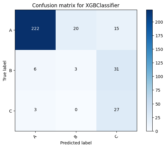
XGBClassifier for dataset A: 0.8961748633879781
XGBClassifier for dataset B: 0.764525993883792
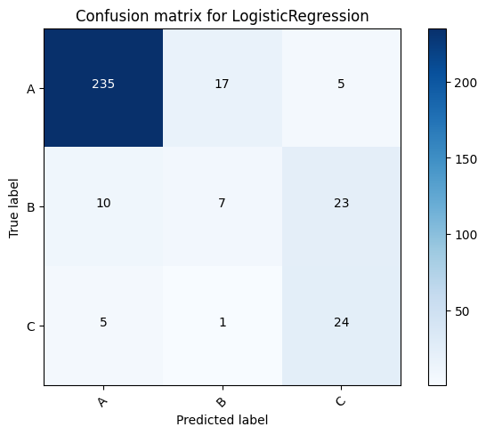
LogisticRegression for dataset A: 0.8633879781420765
LogisticRegression for dataset B: 0.7951070336391437
VotingClassifier for dataset A: 0.8961748633879781
VotingClassifier for dataset B: 0.8195718654434251

class_names = ['A', 'B', 'C']
voting_clf.fit(X_train_A, y_train_A)
y_pred_A = clf.predict(X_test_A)
cnf_matrix = confusion_matrix(y_test_A, y_pred_A)
np.set_printoptions(precision=2)
plt.figure()
plot_confusion_matrix(cnf_matrix, classes=class_names,
                      title='Confusion matrix for ' + clf.__class__.__name__)
plt.show()

Confusion matrix, without normalization
[[130   0   2]
 [  4  11  11]
 [  1   1  23]]

Second case: Training using all of the data from Dataset A

So far we have used 75% of Dataset A to train the data and 25% to test it. Here, we used all of the data from Dataset A to train, and then test it on Dataset B.

from sklearn.ensemble import RandomForestClassifier
from sklearn.ensemble import VotingClassifier
from sklearn.linear_model import LogisticRegression
from sklearn.svm import SVC
from sklearn.neighbors import KNeighborsClassifier
from xgboost import XGBClassifier
from sklearn.neural_network import MLPClassifier
from sklearn.naive_bayes import GaussianNB
from sklearn.ensemble import AdaBoostClassifier

lr_clf = LogisticRegression(max_iter=10000)
svm_clf = SVC(probability=True)
knn_clf = KNeighborsClassifier()
xgb_clf = XGBClassifier(learning_rate=0.01, n_estimators=300, max_depth=3, subsample=0.7)
mlp_clf = MLPClassifier(hidden_layer_sizes=(100,), max_iter=1000)
nb_clf = GaussianNB()
#ada_clf = AdaBoostClassifier(n_estimators=50, learning_rate=0.003)

voting_clf = VotingClassifier(
  estimators=[#('nn', mlp_clf),
              #('svc', svm_clf),
              ('knn', knn_clf), #('ada', ada_clf),('nb', nb_clf)
              ('xgb', xgb_clf), ('lr', lr_clf)],
  voting='hard')
voting_clf.fit(X_A, y_A)

VotingClassifier(estimators=[('knn', KNeighborsClassifier()),
                             ('xgb',
                              XGBClassifier(base_score=None, booster=None,
                                            callbacks=None,
                                            colsample_bylevel=None,
                                            colsample_bynode=None,
                                            colsample_bytree=None,
                                            early_stopping_rounds=None,
                                            enable_categorical=False,
                                            eval_metric=None,
                                            feature_types=None, gamma=None,
                                            gpu_id=None, grow_policy=None,
                                            importance_type=None,
                                            interaction_constraints=None,
                                            learning_rate=0.01, max_bin=None,
                                            max_cat_threshold=None,
                                            max_cat_to_onehot=None,
                                            max_delta_step=None, max_depth=3,
                                            max_leaves=None,
                                            min_child_weight=None, missing=nan,
                                            monotone_constraints=None,
                                            n_estimators=300, n_jobs=None,
                                            num_parallel_tree=None,
                                            predictor=None, random_state=None, ...)),
                             ('lr', LogisticRegression(max_iter=10000))])

In a Jupyter environment, please rerun this cell to show the HTML representation or trust the notebook.
On GitHub, the HTML representation is unable to render, please try loading this page with nbviewer.org.

from sklearn.metrics import accuracy_score

for clf in (#mlp_clf, svm_clf, #ada_clf,
            knn_clf, xgb_clf, lr_clf, #nb_clf,
            voting_clf):
    clf.fit(X_A, y_A)
    y_pred_B = clf.predict(X_B)
    print(clf.__class__.__name__ + " for dataset B:", accuracy_score(y_B, y_pred_B))

KNeighborsClassifier for dataset B: 0.8379204892966361
XGBClassifier for dataset B: 0.7706422018348624
LogisticRegression for dataset B: 0.8134556574923547
VotingClassifier for dataset B: 0.8256880733944955

The code below is a function to visualize the confusion matrix

from sklearn.metrics import confusion_matrix
import itertools
def plot_confusion_matrix(cm, classes, normalize=False, cmap=plt.cm.Blues, title='Confusion matrix'):
    if normalize:
        cm = cm.astype('float') / cm.sum(axis=1)[:, np.newaxis]
        print("Normalized confusion matrix")
    else:
        print('Confusion matrix, without normalization')
    print(cm)

    plt.imshow(cm, interpolation='nearest', cmap=cmap)
    plt.title(title)
    plt.colorbar()
    tick_marks = np.arange(len(classes))
    plt.xticks(tick_marks, classes, rotation=45)
    plt.yticks(tick_marks, classes)

    fmt = '.2f' if normalize else 'd'
    thresh = cm.max() / 2.
    for i, j in itertools.product(range(cm.shape[0]), range(cm.shape[1])):
        plt.text(j, i, format(cm[i, j], fmt),
                 horizontalalignment="center",
                 color="white" if cm[i, j] > thresh else "black")

    plt.tight_layout()
    plt.ylabel('True label')
    plt.xlabel('Predicted label')

Confusion Matrix:

class_names = ['A', 'B', 'C']

for clf in (#mlp_clf, svm_clf, #ada_clf,
            knn_clf, xgb_clf, lr_clf, #nb_clf,
            voting_clf):
    clf.fit(X_A, y_A)
    y_pred_B = clf.predict(X_B)
    cnf_matrix = confusion_matrix(y_B, y_pred_B)
    np.set_printoptions(precision=2)
    plt.figure()
    plot_confusion_matrix(cnf_matrix, classes=class_names,
                          title='Confusion matrix for ' + clf.__class__.__name__)
    plt.show()

Confusion matrix, without normalization
[[245   8   4]
 [ 11  11  18]
 [  8   4  18]]

Confusion matrix, without normalization
[[222  20  15]
 [  6   3  31]
 [  3   0  27]]

Confusion matrix, without normalization
[[235  17   5]
 [ 10   7  23]
 [  5   1  24]]

Confusion matrix, without normalization
[[242  10   5]
 [ 10   3  27]
 [  5   0  25]]

class_names = ['A', 'B', 'C']
voting_clf.fit(X_A, y_A)
y_pred_B = voting_clf.predict(X_B)
cnf_matrix = confusion_matrix(y_B, y_pred_B)
np.set_printoptions(precision=2)
plt.figure()
plot_confusion_matrix(cnf_matrix, classes=class_names,
                      title='Confusion matrix for ' + clf.__class__.__name__)
plt.show()

Confusion matrix, without normalization
[[242  10   5]
 [ 10   3  27]
 [  5   0  25]]